Price Optimization using Econometrics and Calculus

I’ve seen a few people do quick examples of price optimization problems, but one thing I havent seen done is using calculus to obtain the optimal price for a good. In this extremely quick example im going to demonstrate how to do this…

Package Load

library(dplyr)
library(ggplot2)
library(stats) #optimization
library(broom) #tidy model output
library(plotly) #make interactive ggplot visuals

Data

For this exercise we are using beef sales data by quarter that ranges from 1977 - 1999. We can take a quick look at what that looks like to get familiar with our dataset.

head(demand.data)

##   Year Quarter Quantity    Price
## 1 1977       1  22.9976 142.1667
## 2 1977       2  22.6131 143.9333
## 3 1977       3  23.4054 146.5000
## 4 1977       4  22.7401 150.8000
## 5 1978       1  22.0441 160.0000
## 6 1978       2  21.7602 182.5333

Exploration

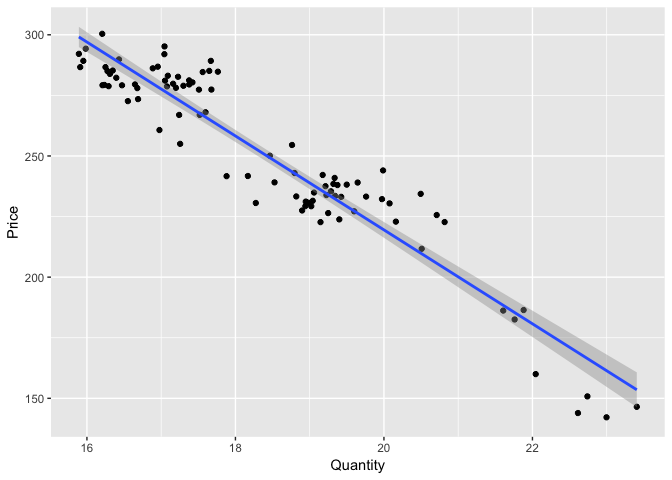
Here we are just taking a look at the relationship between price and demand for beef - we see a pretty clear negative relationship here.

demand.data %>%
  ggplot(aes(Quantity, Price)) +
    geom_point() +
    geom_smooth(method = "lm")

plot1

Estimating the demand equation

This is something that’s extremely important to note… We are dealing with an extremely simplistic dataset. The negative relationship between price and demand may not always be as clear as we saw in the above plot. In a real application I can guarantee you it wont be this easy to uncover the relationship between price and demand. This is why correctly specifying our model is of EXTREME importantce. The math to determine the optimal price from our estimated model is super easy compared to this. There’s going to be many other variables that influence demand such as seasonality, price of substitute goods etc which impact the demand for beef. If we control for the correct varaibes we should always uncover a negative relationship.

demand.model <- lm(Quantity ~ Price, data = demand.data)

For the sake of brevity, we are going to assume that this model is simply amazing. We would normally be checking our model diagnostics, thinking from a theory standpoint if we have the correct variables in our model violating any of the Gauss-markov assumptions of regression etc…

How to evaluate the model is any good or not will be a post for another day.

Demand Equation

As we see from our model output above, now we have a demand equation.

$TR = \beta_0P + \beta_1P^2$

Qdemand = 30.05 - 0.04 x Price

In english this says, for every $1 increase in price, on average the quantity of beef sales will decrease by .04 (units?) whatever a unit of beef is…

Now we are going to save that equation as a function for later use

demand.equation <- function(x){
  (x-80)*(30.05-.0465*x)
}

Here comes the calculus…

Sir Issac Newton would be proud!…

Now this is where the example is going to diverge from what I’ve seen others do… And by all means the way others have done it is completely correct - there’s 1,000 ways to skin a sheep. What I’ve seen typically done is people will generate a vector of arbitrary prices, say $0 - $1,000 and evaluate their demand equation at each price and see what the estimated revenue will be. This definitely works, but in my opinion there’s a far more efficient and sophisticated way to solve this problem. After all, I dont want to let all those hours studying math go to waste.

If you remember back to your calculus classes - one of the main focuses is derivatives. Now, here’s a real life, useful application of all that hard work.

In this instance we can take the first derivative of our demand function with respect to price, set that equation equal to 0 and solve for price. Setting the function = 0 and solving will yield what the revenue maximizing price will be.

Setting it equal to 0 means the slope of the line at the price is flat… We’ll see an example below. Lucky for us, we dont have to handwrite our math and we have this optimize function out of the stats package that will do all the heavy lifting for us.

profit.max <- stats::optimize(demand.equation, lower = 0, upper = 500, maximum = TRUE)
print(profit.max$maximum)

## [1] 363.1183

Using the above function, we see that our revenue maximizing price is $363.

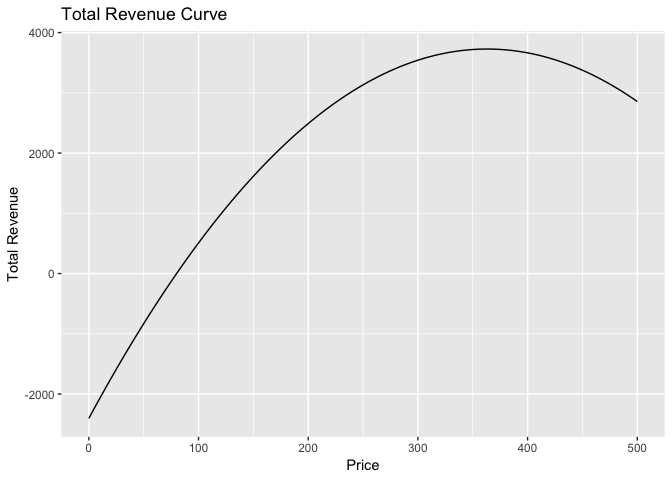
Total Revenue Curve

In this particular example we are optimizing price to maximize revenue. I understand that’s not always the metric that we are trying to maximize. We can also extend this and maximize profit, for that we will just need to include cost in our equation and obtain a profit function rather than just a total revenue function. (just a bit more algebra)

  ggplot(data.frame(price = 0:500), aes(price)) +
    stat_function(fun = demand.equation, geom = 'line') +
    labs(title = "Total Revenue Curve", x = "Price", y = "Total Revenue")

plot2